Normalized Cross-Entropy
This post explores a normalized version of binary cross-entropy loss in attempt to remove the effect of the prior (class imbalance within the dataset) on the resulting value.
Context
A common machine-learning task within the advertising domain is modeling user-ad click propensity.
\[P(click \space | \space user,ad) \tag 1 \label 1\]The Occam’s Razor problem solving approach tells us that starting out with a simple model is usually a good first start. We begin by applying a well-studied generalized linear model (GLM), logistic regression (LR), which models a binary response random variable. It outputs a probability, $\hat p$, for predicted membership to the positive class as a deterministic function, $h$, of some feature embedding, $\textbf x$, parameterized by, $\boldsymbol{\hat \theta}$, our current hypothesis.
\[\hat p=\\ P(\hat y=1 \space | \space \textbf x;\boldsymbol{\hat \theta})=\\ h_\boldsymbol{\hat \theta}(\textbf{x}) \tag 2 \label 2\]The goal of learning is to approximate nature’s hypothetical target function which maps a full-relationship for some inputs to a true target value. Whatever your view on reality or spin on probability, lets assume a true probabilistic binary generative process so that we can draw an analog to the LR model. We express nature by recycling notation from \ref{2}.
\[p=\\ P(y=1 \space | \space \textbf x;\boldsymbol{\theta})=\\ h_\boldsymbol{\theta}(\textbf{x}) \tag 3 \label 3\]Fueled by data, LR learns by iteratively adjusting its model parameters, $\boldsymbol{\hat \theta}$, so that its predictions are better aligned to nature (what’s been observed). Specialized algorithms can be applied to guide an informative search through an infinite-sized hypothesis (parameter) space to find a hypothesis (or the parameters) that best reflects reality.
Challenges may arise from model complexity, measurement noise, and insufficient data. If our model is unable to capture the complexity of the target function it will fail to generalize. If our model is overly complex, it may mistakenly learn the noise in our training data and fail to generalize. Moreover, if the data is not predictive, of low-quality, or is missing, there wouldn’t be much to learn; garbage in, garbage out.
Definition
We must carefully select an evaluation metric which enables us to measure and compare model performance. We evaluate our model’s generalization capabilities on a test or holdout-set of data for which the model has not been exposed to during training. Since we know if the user has clicked or not, we can assess the model’s predictions against reality. A good model will be better aligned to reality.
After researching many metrics, we consider Normalized Cross-Entropy (NCE).
Facebook research
Normalized Cross-Entropy is equivalent to the average log-loss per impression divided by what the average log-loss per impression would be if a model predicted the background click through rate (CTR) for every impression. [1]
Variables
- $N$ is the size of the test-set (total number of ad-impressions).
- $CTR$ is the observed click-through rate (proportion of clicks to ad-impressions) in the test-set.
- $\hat p$, where $\{ \hat p \in \mathbb{R} \space | \space 0 \le \hat p \le 1\}$, is our model’s predicted probability score (that the user will click).
- $p$, where $p \in \{0, 1\}$, is the observed probability score (often referred to as the label).
- 1 indicates that the user did click (the probability of click is 1 since we’re certain they clicked); $P(click \space | \space user,ad)=1$.
- 0 indicates that the user didn’t click (the probability of click is 0 since we’re certain they didn’t click); $P(click \space | \space user,ad)=0$.
Equation
\[NCE=\\ \frac { -\frac{1}{N}\sum_{i=1}^N (p_i \cdot ln(\hat p_i) + (1-p_i) \cdot ln(1-\hat p_i)) } { -\frac{1}{N}\sum_{i=1}^N (p_i \cdot ln(CTR) + (1-p_i) \cdot ln(1-CTR)) } \tag 4 \label 4\]What is log-loss?
In mathematical optimization and decision theory, a loss function or cost function is a function that maps an event or values of one or more variables onto a real number intuitively representing some “cost” associated with the event. An optimization problem seeks to minimize a loss function. [7]
Log-loss can be derived from several schools of thought. In the case of binary classification, derivations yield equivalence.
Probability Theory derivation
Bernoulli
A user’s true click propensity for a single ad-impression, $Y$, follows a Bernoulli distribution. Since, the user will click with some probability, $p$, and not-click with the complement probability, $1-p$, the probability mass function (PMF) can be expressed in-line.
\[Y \sim Bernoulli(p)=\\ p^k(1-p)^{1-k} \space\space\space for \space k \in \{0, 1\} \tag 5 \label 5\]GLMs relate a linear predictor to the conditional expected value of the estimated response variable by applying a link function. LR estimates the expected value of a Bernoulli-distributed response variable by piping a linear predictor through an inverse logit link function.
\[\mathbb{E}[\hat Y|X]=\\ \hat p=\\ g^{-1}(X \theta)=\\ h_{\theta}(X) \tag 6 \label 6\]The linear predictor is a function of some feature embedding, $\textbf x$, parameterized by a model hypothesis, $\boldsymbol{\hat \theta}$. Per equation \ref{2}, $h$ represents the final output, that is, after the linear transform’s output passes through the link function.
\[\hat Y|X \sim Bernoulli(\hat p)=\\ Bernoulli(h_\boldsymbol{\hat \theta}(\textbf x)) \tag 7 \label 7\]In order to estimate $p$ we invoke maximum likelihood estimation over our training set.
In statistics, maximum likelihood estimation (MLE) is a method of estimating the parameters of a probability distribution by maximizing a likelihood function, so that under the assumed statistical model the observed data is most probable. [8]
In order to find the maximum likelihood estimate, we must define the likelihood function for our data and then maximize it. The value $\hat p$ takes at the maximum is our maximum likelihood estimate for the true parameter $p$.
In statistics, the likelihood function (often simply called the likelihood) measures the goodness of fit of a statistical model to a sample of data for given values of the unknown parameters. [9]
Generally, for a design-matrix (rows are training examples and columns are features), $\textbf X$, and true observation matrix (associated labels), $\textbf Y$, we define the likelihood function as the probability of the joint distribution of the training data as a function of the parameter(s) being estimated, in our case, $\hat{\boldsymbol{\theta}}$.
\[\mathcal{L}(\hat{\boldsymbol{\theta}}| \textbf X_{m \space \times \space f},\textbf Y_{m \space \times \space 1})=\\ P(\textbf X_{m \space \times \space f},\textbf Y_{m \space \times \space 1}; \hat{\boldsymbol{\theta}}) \tag 8 \label 8\]Assuming a training set of size $M$ ad-impressions that are conditionally independent (but not identically distributed, i.e., different expected values) Bernoulli trials, we can calculate the joint probability mass function for a given parameter, $\hat{\boldsymbol{\theta}}$.
\[P(\textbf X_{m \space \times \space f},\textbf Y_{m \space \times \space 1}; \hat{\boldsymbol{\theta}})=\\ \prod_{i = 1}^{M} h_\boldsymbol{\hat \theta}(\textbf{x}_i)^{y_i} (1-h_\boldsymbol{\hat \theta}(\textbf{x}_i))^{1-y_i} \tag 9 \label 9\]The value of the joint probability mass function may get very small as multiplying small numbers by small numbers result in even smaller numbers. At some point, we may hit computational floating-point arithmetic underflow errors. We can instead maximize the log of the likelihood. One benefit of the log function is that it is a monotonically increasing function, i.e., the log-transformation preserves ordering and doesn’t change where the maximum is. Computationally, another benefit of the log function is that it turns repeated multiplication into a summation. The list of logarithmic identities is a good refresher.
\[ln(P(\textbf X_{m \space \times \space f},\textbf Y_{m \space \times \space 1}; \hat{\boldsymbol{\theta}}))=\\ \sum_{i = 1}^{M} {y_i} \cdot ln(h_\boldsymbol{\hat \theta}(\textbf{x}_i)) + (1-y_i) \cdot ln(h_\boldsymbol{\hat \theta}(\textbf{x}_i)) \tag {10} \label {10}\]Most mathematical optimization algorithms implemented in software are minimizers. Gradient descent, a well-suited minimization algorithm, applies an iterative first-order hill-descent routine which converges at a local minimum. In order to find the maximum of the log-likelihood function, we instead find the minimum of the negative log-likelihood. Finally, we normalize by the number of examples in the summation yielding the average log-loss. An added benefit to the normalization is that the number of examples fed in is not a factor, i.e., if we wanted to compare the average log-loss over some batch size.
\[-\frac{1}{M}ln(P(\textbf X_{m \space \times \space f},\textbf Y_{m \space \times \space 1}; \hat{\boldsymbol{\theta}}))=\\ -\frac{1}{M}\sum_{i = 1}^{M} {y_i} \cdot ln(h_\boldsymbol{\hat \theta}(\textbf{x}_i)) + (1-y_i) \cdot ln(h_\boldsymbol{\hat \theta}(\textbf{x}_i)) \tag {11} \label {11}\]Binomial
Through a similar but slightly different point of view, the overall or prior click propensity follows a Binomial distribution. Its PMF yields the probability of getting exactly $k$ clicks in a series of $n$ independently and identically distributed (i.i.d) ad-impressions (Bernoulli trials) under one common click propensity, $p$.
\[P(k;n,p) \sim\\ Binomial(n, k, p)=\\ \binom{n}{k} p^k(1-p)^{n-k} \tag {12} \label {12}\]The binomial coefficient scales the value of the PMF by the number of combinations that $k$ clicks could have occurred within a series of $n$ ad-impressions. Since it is a constant, it won’t have any effect on the maximum and can be safely ignored. We’re then left with a series of i.i.d Bernoulli trials to which we can apply very similar mathematics from the Bernoulli derivation above. Naturally, the Binomial MLE resolves to the prior CTR, $\frac{k}{n}$. In other words, the Binomial likelihood is maximal under a fixed number of trials at the observed success rate.
Information Theory derivation
Information theory studies the quantification, storage, and communication of information. It was originally proposed by Claude Shannon in 1948 to find fundamental limits on signal processing and communication operations such as data compression, in a landmark paper titled “A Mathematical Theory of Communication”. [10]
Information content
Given random variable $X$ with PMF $P_{X}(x)$, we can measure the information, $I_X$, of outcome, $x$, as the log (usually base $e$, $2$, or $10$) inverse probability of that outcome.
\[I_X(x)=\\ ln(\frac{1}{P_X(x)}) \tag {13} \label {13}\]Why the inverse probability?
The inverse probability or “surprisal” for a given outcome is larger when the outcome is less likely
and smaller when the outcome is more likely. In other words, events that occur very frequently
don’t carry as much information as events that occur rarely. Intuitively, less-likely events
carry more information because they inform us that not only they’ve occurred but that their more
likely counterparts didn’t occur. For example, when drawing a letter randomly from the 5 character
string ABBBB, the probability of drawing an A is $0.2$ while the probability of drawing a B is
$0.8$. If we draw A, we can eliminate $\frac{1}{.2}=5$ characters, that is, the A because it
occurred and all of the Bs because we know they didn’t occur. If we draw B, we can eliminate
$\frac{1}{.8}=1.25$ characters, that is, the one and only A because we know it didn’t occur and
a quarter of the Bs because we know one of them occurred. Since, drawing an A allows us to
eliminate more characters from the string, it carries more information.
Why the logarithmic transform?
Directly from Claude Shannon’s white-paper.
The logarithmic measure is more convenient for various reasons:
- It is practically more useful. Parameters of engineering importance such as time, bandwidth, number of relays, etc., tend to vary linearly with the logarithm of the number of possibilities. For example, adding one relay to a group doubles the number of possible states of the relays. It adds 1 to the base 2 logarithm of this number. Doubling the time roughly squares the number of possible messages, or doubles the logarithm, etc.
- It is nearer to our intuitive feeling as to the proper measure. This is closely related to (1) since we intuitively measures entities by linear comparison with common standards. One feels, for example, that two punched cards should have twice the capacity of one for information storage, and two identical channels twice the capacity of one for transmitting information.
- It is mathematically more suitable. Many of the limiting operations are simple in terms of the logarithm but would require clumsy restatement in terms of the number of possibilities. [11]
Entropy
Entropy, $H$, is the expected value of information. For a discrete random variable, $X$, it is the weighted average of the information of each of its outcomes.
\[H(X)=\\ \mathbb{E}_{x \sim P}[I_X]=\\ \sum_{i}^{N}P(x_i) \cdot ln(\frac{1}{P(x_i)})=\\ -\sum_{i}^{N}P(x_i) \cdot ln(P(x_i)) \tag {14} \label {14}\]Entropy can be interpreted as a measure of chaos and/or uncertainty in that it is maximized when outcomes are equiprobable, i.e., carry the same amount of information (uniform PMF), and minimized or $0$ when outcomes are certain. In the case of a binary random variable, it is maximal when each outcome has a $0.5$ probability mass. It is minimized or $0$ when one of the outcomes have a $1.0$ probability (the other having a $0.0$ probability). We can measure entropy as the average number of bits required to encode the information content of a random variable by substituting $log_2$ for $ln$ into \ref{14}.
\[-0.5 \cdot log_2(0.5)-0.5 \cdot log_2(0.5)=1 \tag {15} \label {15}\] \[-1.0 \cdot log_2(1.0)-0.0 \cdot log_2(0.0)=\\ -0.0 \cdot log_2(0.0)-1.0 \cdot log_2(1.0)=0 \tag {16} \label {16}\]On average, we need one bit to represent a fair coin and no bits to represent a double-headed or double-tailed coin because no matter what, we know the outcome. The lack of stochasticity implies that we don’t need to flip the coin as we know the outcome a priori.
Cross-entropy
Cross-entropy (CE) measures the expected value of information for random variable, $X$, with PMF, $P$, using a coding scheme optimized for another, $Y$, with PMF, $Q$, over the same support, i.e., set of outcomes/events.
\[H(X,Y)=\\ \mathbb{E}_{x \sim P}[I_Y]=\\ \sum_{i}^{N}P(x_i) \cdot ln(\frac{1}{Q(x_i)})=\\ -\sum_{i}^{N}P(x_i) \cdot ln(Q(x_i)) \tag {17} \label {17}\]If $X = Y$, then CE resolves to entropy. If $X \neq Y$, CE can be expressed in terms of entropy and Kullback–Leibler divergence.
\[H(X,Y)=\\ H(X) + D_{KL}(X||Y) \tag {18} \label {18}\]Kullback–Leibler divergence
Assuming random variables $X$ and $Y$ with respective PMFs $P$ and $Q$ over common support, Kullback–Leibler divergence (KLD) is the expected logarithmic difference between the two or equivalently, the expected logarithm over likelihood ratios.
\[D_{KL}(X||Y) =\\ \mathbb{E}_{x \sim P}[ln(\frac{P(x)}{Q(x)})]=\\ \sum_{i}^{N}P(x_i) \cdot ln(\frac{P(x_i)}{Q(x_i)}) \tag {19} \label {19}\]It’s an asymmetric measure with a minimal value at 0, meaning the distributions are identical. The inequality implies that KLD is not a distance metric, hence the word “divergence” in its name.
\[D_{KL}(X||Y) \neq D_{KL}(Y||X) \tag {20} \label {20}\]Based on the definition of CE in \ref{18}, KLD can be understood as the average extra information required to be encoded since we’ve calculated the entropy of $X$ using a potentially suboptimal encoding scheme (from $Y$). Notice, again, if the KLD is $0$, then the CE of $X$ is just the entropy of $X$ and that if it is $> 0$ then the CE of $X$ is the entropy of $X$ plus some additional divergence, which yields a suboptimal encoding for $X$.
Minimizing cross-entropy / Kullback–Leibler divergence
LR is a supervised learning algorithm because it learns to map inputs to outputs based on training example input-output pairs. For each training example, the outcome has already been observed, i.e., the probability that the user clicked is either $1.0$ or $0.0$. LR learns by comparing its prediction to the respective outcome and correcting itself. Since both prediction and outcome binary probability distributions cover the same support, CE applies as a measure of how close the prediction distribution is to the outcome distribution.
The entropy of an observed outcome is $0$ because the act of observation collapses the probabilistic nature of what could have happened, e.g., if a user clicked, the entropy is $0$ because there is complete certainty the event has occurred. The same applies if the user decided not to click. See \ref{16}. Since the entropy of the reference distribution, $X$, is $0$, we can eliminate $H(X)$ from \ref{18} when calculating the CE. Thus, in this case, minimizing CE is equivalent to minimizing KLD.
\[H(X,Y)=\\ 0 + D_{KL}(X||Y)=\\ D_{KL}(X||Y) \tag {21} \label {21}\]Cross-entropy loss
There’s no need to write out the mathematics for calculating CE loss over $M$ training examples because we’ve already derived it via probability theory. Minimizing the average CE of $M$ training examples is equivalent to minimizing the negative log-likelihood of those $M$ training examples under the Bernoulli model. That’s two schools of thought arriving at the same conclusion with the same equation :P!
If the connection between the two isn’t obvious, compare and contrast \ref{11} and \ref{17}. What happens if we calculate the CE between the model’s prediction and the observed outcome (\ref{22}/\ref{23})? What happens if we do that for all $M$ training examples and then take the average?
Visualizing…
Log-loss / cross-entropy
CE is applied during model training/evaluation as an objective function which measures model performance. The model learns to estimate Bernoulli distributed random variables by iteratively comparing its estimates to natures’ and penalizing itself for more costly mistakes, i.e., the further its prediction is from what has been observed, the higher the cost that is realized. For simplicity, let’s assume observed and estimated binary response random variables, $Y$ and $\hat Y$ with respective PMFs $P$ and $Q$, that represent the modeled propensity and outcome for some user clicking on some ad.
\[H(Y, \hat Y)=\\ -\sum_{i}^{N}P(x_i) \cdot ln(Q(x_i)) \tag {22} \label {22}\]Since $P(x_i)$ is always either $1.0$ or $0.0$, as it is the observed outcome, CE can be expanded as the sum of two mutually exclusive negated log functions of which only one gets activated according to the observed outcome. Since our model outputs the probability of a click as $Q(x)$, the complement probability of not clicking is $1-Q(x)$.
\[-((P(x) \cdot ln(Q(x))) +\\ ((1-P(x)) \cdot ln(1-Q(x))))=\\ \left \{ \begin{aligned} &-ln(Q(x)), && P(x)=1.0 \\ &-ln(1-Q(x)), && P(x)=0.0 \end{aligned} \right. \tag {23} \label {23}\]Perhaps a bit cleaner, the PMFs can be replaced with $p$ and $\hat p$ from \ref{3} and \ref{2}.
\[-((p \cdot ln(\hat p)) +\\ ((1-p) \cdot ln(1-\hat p)))=\\ \left \{ \begin{aligned} &-ln(\hat p), && p=1.0 \\ &-ln(1-\hat p), && p=0.0 \end{aligned} \right. \tag {24} \label {24}\]Fig. 1
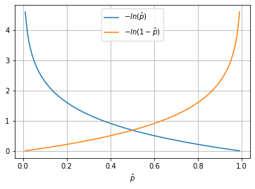
Fig 1. [13] shows the cost our model realizes when the outcome is a click (in blue) and not a click (in orange).
If the outcome is a click (outcome probability of a click is $1.0$), and the model predicts a probability of $1.0$, the model realizes a cost of $0.0$, i.e., the model isn’t penalized as the prediction is perfectly reflective of the outcome. In the case that the model predicts anything less than $1.0$, it will realize a cost that grows exponentially as the prediction moves further away from $1.0$.
If the outcome is not a click (outcome probability of a click is $0.0$), the reflection of the same logic applies, i.e., the model must predict $0.0$ to realize a cost of $0.0$ and that cost grows exponentially as the model’s prediction moves further away from $0.0$.
Normalized log-loss / cross-entropy
Click-through rate entropy
The NCE (\ref{4}) denominator can be expressed as the entropy (\ref{14}) of the prior CTR which is equivalent to the average log-loss if the model always predicted the CTR.
\[-\frac{1}{N}\sum_{i=1}^N (p_i \cdot ln(CTR) + (1-p_i) \cdot ln(1-CTR))=\\ -\frac{1}{N}\sum_{i=1}^N p_i \cdot ln(CTR)-\frac{1}{N}\sum_{i=1}^N(1-p_i) \cdot ln(1-CTR)=\\ -\sum_{i=1}^N\frac{p_i \cdot ln(CTR)}{N}-\sum_{i=1}^N\frac{(1-p_i) \cdot ln(1-CTR)}{N}=\\ -(CTR \cdot ln(CTR) + (1-CTR) \cdot ln(1-CTR)) \tag {25} \label {25}\]Fig. 2
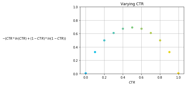
Fig. 2 [13] shows entropy as a function of CTR. It is maximized at a CTR of $0.5$ when clicking is just as likely as not clicking. The more the CTR drifts from $0.5$, in either direction, the resulting entropy symmetrically decreases. At a CTR of $0.0$ or $1.0$, the entropy would be $0.0$ as there would be complete certainty of the outcome from the data, e.g., only clicks or no clicks at all.
Fig. 3
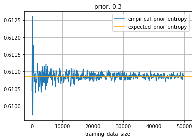
Fig. 3 [14] shows the result of a simulating \ref{25} while varying training set size. The CE of each training example outcome, $\sim Bernoulli(0.3)$, and prediction, $0.3$ (prior), is averaged over the $N$ prediction-outcome pairs. As the size of the training set increases, the empirical cross-entropy converges to the expected prior entropy of $-.3 \cdot log(.3)-(1-.3) \cdot log(1-.3)=.610$.
Fig. 4
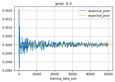
Fig. 4 [14] shows the result of a simulating the proportion of observations that resulted in a positive label while varying training set size. The proportion converges to the expected value as the number of trials or size of the training set increases. Since each outcome for in a given training set size follows $Bernoulli(0.3)$, we’d expect the sampled proportion to converge to $0.3$ as we simulate larger training set sizes.
Both simulations are manifestations of the law of large numbers. As the prior converges, so does the entropy of the prior since mathematically (\ref{25}), it is dependent on it.
Baseline model
When doing supervised learning, a simple sanity check consists of comparing one’s estimator against simple rules of thumb.
- stratified: generates random predictions by respecting the training set class distribution.
- most_frequent: always predicts the most frequent label in the training set.
- prior: always predicts the class that maximizes the class prior (like most_frequent) and predict_proba returns the class prior.
- uniform: generates predictions uniformly at random.
- constant: always predicts a constant label that is provided by the user. [12]
NCE is defined (see \ref{4}) as the predictive log-loss normalized by the log-loss of a baseline prior model, i.e., a model which always outputs the probability of a click as the observed CTR. One way to visualize the behavior of the normalization is to restrict the model’s predictions to various hypothetical CTRs.
\[\hat p = \hat{CTR} \tag {26} \label {26}\]That constraint means our model’s predictions are a constant and NCE can be broken into two mutually exclusive terms and visualized separately.
\[NCE=\\ \frac { -\frac{1}{N}\sum_{i=1}^N (p_i \cdot ln(\hat p_i) + (1-p_i) \cdot ln(1-\hat p_i)) } { -\frac{1}{N}\sum_{i=1}^N (p_i \cdot ln(CTR) + (1-p_i) \cdot ln(1-CTR)) }=\\ \frac { -\frac{1}{N}\sum_{i=1}^N (p_i \cdot ln(\hat{CTR}) + (1-p_i) \cdot ln(1-\hat{CTR})) } { -\frac{1}{N}\sum_{i=1}^N (p_i \cdot ln(CTR) + (1-p_i) \cdot ln(1-CTR)) }=\\ \frac { -\frac{1}{N}\sum_{i=1}^N p_i \cdot ln(\hat{CTR}) - \frac{1}{N}\sum_{i=1}^N (1-p_i) \cdot ln(1-\hat{CTR}) } { -\frac{1}{N}\sum_{i=1}^N p_i \cdot ln(CTR) - \frac{1}{N}\sum_{i=1}^N (1-p_i) \cdot ln(1-CTR) }=\\ \frac { -\sum_{i=1}^N \frac{p_i \cdot ln(\hat{CTR})}{N} - \sum_{i=1}^N \frac{(1-p_i) \cdot ln(1-\hat{CTR})}{N} } { -\sum_{i=1}^N \frac{p_i \cdot ln(CTR)}{N} - \sum_{i=1}^N \frac{(1-p_i) \cdot ln(1-CTR)}{N} }=\\ \frac { -(CTR \cdot ln(\hat{CTR}) + (1-CTR) \cdot ln(1-\hat{CTR})) } { -(CTR \cdot ln(CTR) + (1-CTR) \cdot ln(1-CTR)) }=\\ \frac { CTR \cdot ln(\hat{CTR}) } { CTR \cdot ln(CTR) + (1-CTR) \cdot ln(1-CTR) }\\ + \frac { (1-CTR) \cdot ln(1-\hat{CTR}) } { CTR \cdot ln(CTR) + (1-CTR) \cdot ln(1-CTR) } \tag {27} \label {27}\]Fig. 5
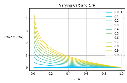
Fig. 6
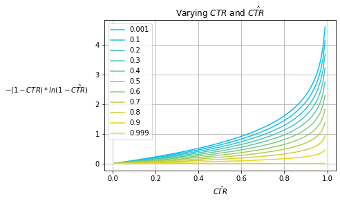
Fig. 7
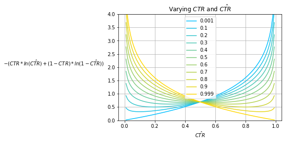
Fig. 7 shows the CE of various baseline prior models that always predict $\hat{CTR}$ for various observed prior $CTR$s; Fig. 5 and Fig. 6 show its decomposed summands. The effect of the observed prior $CTR$ manifests as a scaling factor applied to each of the logarithms which is exacerbated for very high and very low $CTR$s. Notice that the minima for each $CTR$ curve exists at $\hat{CTR}=CTR$ while the actual minimum value changes over various $CTR$s.
Note that Fig. 7 only captures the performance of baseline prior models which are relatively weak in terms of model performance. In practice, a good model will outperform baseline measures as it isn’t constrained to only predicting some fixed $\hat{CTR}$.
Fig. 8
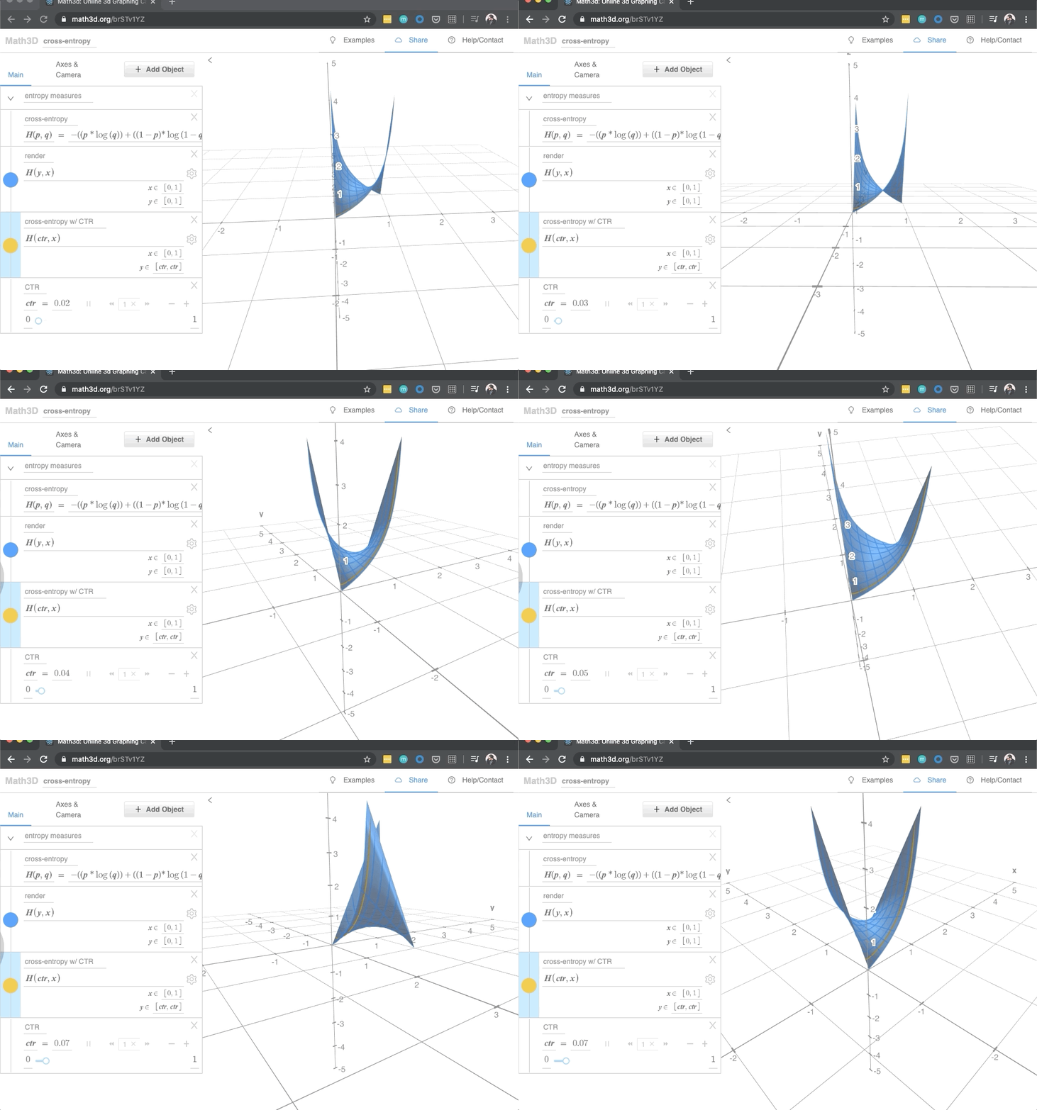
Fig. 8 is a GIF of a 3D rendering of the binary CE function. Notice the two minimum values of $0.0$ when $x$ and $y$ are both either $0.0$ or $1.0$. The animated yellow line is a 3D variation of Fig. 7. Click here to reproduce and interact within your web browser.
Fig. 9
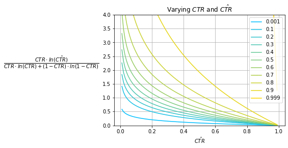
Fig. 10
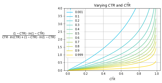
Fig. 11
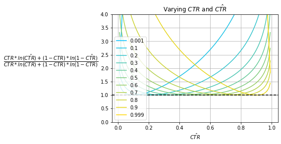
Fig. 11 shows the NCE of various baseline prior models that always predict $\hat{CTR}$ for various observed prior $CTR$s; Fig. 9 and Fig. 10 show its decomposed summands. Notice that the effect of the $CTR$ is removed. For each $CTR$ curve, while the minima still exists at $\hat{CTR}=CTR$, the minimum value is $1.0$ and this is the case for all $CTR$s.
Note that Fig. 11 only captures the performance of baseline prior models which are relatively weak in terms of model performance, i.e., the best model will produce a score of $1.0$. In practice, a good model will outperform baseline measures as it isn’t constrained to only predicting some fixed $\hat{CTR}$. This pushes the NCE theoretical lower bound down to $0.0$ from $1.0$.
Fig. 12
Fig. 12 is a GIF of a 3D rendering of the binary NCE (rainbow) and CE (blue) functions. Notice the same two minimum values of $0.0$ when $x$ and $y$ are both either $0.0$ or $1.0$. The animated yellow line is a 3D variation of Fig. 7. The animated orange line is a 3D variation of Fig. 11. Click here to reproduce and interact within your web browser.
Special Thanks
A special thanks to Chris Chudzicki for his mathematics visualization tool, Math3D. It’s an excellent alternative to Desmos that offers support for three-dimensional rendering.
References
[1] X. He, J. Pan, O. Jin, T. Xu, B. Liu, T. Xu, Y. Shi, A. Atallah, R. Herbrich, S. Bowers, and J. Q. n. Candela. Practical lessons from predicting clicks on ads at facebook. https://research.fb.com/wp-content/uploads/2016/11/ practical-lessons-from-predicting-clicks-on-ads-at-facebook.pdf?
[2] J. Yi, Y. Chen, J. Li, S. Sett, and T. W. Yan. Predictive model performance: Offline and online evaluations. https://chbrown.github.io/kdd-2013-usb/kdd/p1294.pdf
[3] Kamelia Aryafar, Devin Guillory, and Liangjie Hong. 2017. An Ensemble-based Approach to Click-Through Rate Prediction for Promoted Listings at Etsy. https://arxiv.org/pdf/1711.01377.pdf
[4] V. Sreenivasan, F. Hartl. Neural Review Ranking Models for Ads at Yelp. https://web.stanford.edu/class/archive/cs/cs224n/ cs224n.1174/reports/2761953.pdf
[5] C. Li, Y. Lu, Q. Mei, D. Wang, S. Pandey. Click-through Prediction for Advertising in Twitter Timeline. http://www-personal.umich.edu/~qmei/pub/kdd2015-click.pdf
[6] X. Ling, W. Deng, C. Gu, H. Zhou, C. Li, F. Sun. Model Ensemble for Click Prediction in Bing Search Ads. https://www.microsoft.com/en-us/research/wp-content/uploads/2017/04/main-1.pdf
[7] https://en.wikipedia.org/wiki/Loss_function
[8] https://en.wikipedia.org/wiki/Maximum_likelihood_estimation
[9] https://en.wikipedia.org/wiki/Likelihood_function
[10] https://en.wikipedia.org/wiki/Information_theory
[11] C. E. Shannon. A Mathematical Theory of Communication. https://web.archive.org/web/19980715013250/http://cm.bell-labs.com/cm/ms/what/ shannonday/shannon1948.pdf
[12] https://scikit-learn.org/stable/modules/model_evaluation.html#dummy-estimators
[13] https://github.com/daniel-deychakiwsky/notebooks/blob/master/experiments/cross_entropy_log_likelihood.ipynb
[14] https://github.com/daniel-deychakiwsky/notebooks/blob/master/simulations/prior_cross_entropy_convergence_sim.ipynb